

JupyterLab is the next-generation user interface for Project Jupyter offering all the familiar building blocks of the classic Jupyter Notebook (notebook, terminal, text editor, file browser, rich outputs, etc.) in a flexible and powerful user interface.
Project Jupyter develops open-source software, open-standards, and services for interactive computing across dozens of programming languages.
The Jupyter Notebook extends the console-based approach to interactive computing in a qualitatively new direction, providing a web-based application suitable for capturing the whole computation process: developing, documenting, and executing code, as well as communicating the results.
The Jupyter Notebook combines two components:
- A web application: a browser-based tool for interactive authoring of documents which combine explanatory text, mathematics, computations and their rich media output.
- Notebook documents: a representation of all content visible in the web application, including inputs and outputs of the computations, explanatory text, mathematics, images, and rich media representations of objects.
JupyterLab is a web-based interactive development environment for Jupyter notebooks, code, and data. JupyterLab is flexible: configure and arrange the user interface to support a wide range of workflows in data science, scientific computing, and machine learning. JupyterLab is extensible and modular: add new functionality or change almost any aspect of how the interface behaves.
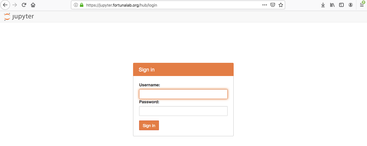
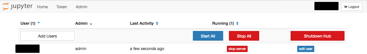
In our lab, JupyterLab is deployed with JupyterHub and then it shows additional menu items in the "File" menu that allow the user to log out or go to the JupyterHub control panel. Therefore, lab members are taken to their JupyterLab interface by default after login, and later on they can access the Hub from their JupyterLab instances.
Jupyter supports over 40 programming languages, including Python, R, Julia, and MatLab. A kernel is a program that runs and introspects the user's code. IPython includes a kernel for Python code, and people have written kernels for several other languages. When Jupyter starts a kernel, it passes it a connection file. You can choose the kernel you want for your notebook depending on the programming language you use to write and run your code.
Jupyter Notebook.
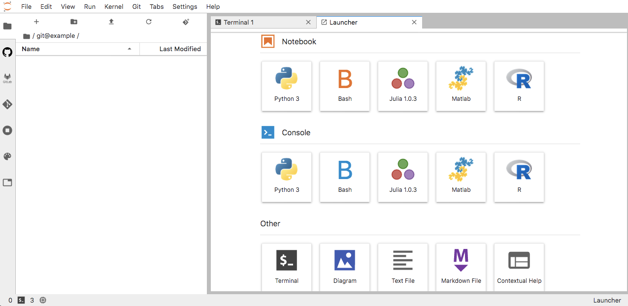
You can create new notebooks from the JupyterLab dashboard with the New Launcher "plus" button, or open existing ones by clicking on their name. You can also drag and drop .ipynb notebooks into the "File Browser" tab.
Creating a new notebook document.
A new notebook may be created at any time using the "File" > "New Notebook" option. The new notebook is created within the same directory and will open in a new browser tab.
Opening notebooks.
An open notebook has exactly one interactive session connected to a kernel, which will execute code sent by the user and communicate back results. This kernel remains active if the web browser window is closed, and reopening the same notebook from the dashboard will reconnect the web application to the same kernel.
Notebook user interface.
When you create a new notebook document, you will be presented with the notebook name, a menu bar, a toolbar and an empty code cell.
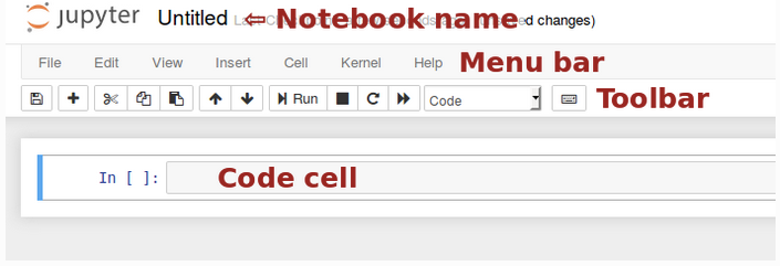
Notebook name:
The name displayed at the top of the page reflects the name of the .ipynb file. Clicking on the notebook name brings up a dialog which allows you to rename it.
Menu bar:
The menu bar presents different options that may be used to manipulate the way the notebook functions.
Toolbar:
The tool bar gives a quick way of performing the most-used operations within the notebook, by clicking on an icon.
Code cell:
The default type of cell; read on for an explanation of cells.
Structure of a notebook document.
The notebook consists of a sequence of cells. A cell is a multiline text input field, and its contents can be executed by using Shift-Enter, or by clicking either the "Play" button in the toolbar, or "Cell" > "Run" in the menu bar. The execution behavior of a cell is determined by the cell's type. There are three types of cells: code cells, markdown cells, and raw cells. Every cell starts off being a code cell, but its type can be changed by using a drop-down on the toolbar (which will be "Code", initially), or via keyboard shortcuts.
Code cells.
A code cell allows you to edit and write new code, with full syntax highlighting and tab completion. The programming language you use depends on the kernel you selected.
When a code cell is executed, code that it contains is sent to the kernel associated with the notebook. The results that are returned from this computation are then displayed in the notebook as the cell's output. The output is not limited to text, with many other possible forms of output are also possible, including figures and tables.
Markdown cells.
You can document the computational process in a literate way, alternating descriptive text with code, using rich text. This is accomplished by marking up text with the Markdown language. The corresponding cells are called Markdown cells. The Markdown language provides a simple way to perform this text markup, that is, to specify which parts of the text should be emphasized (italics), bold, form lists, etc.
If you want to provide structure for your document, you can use markdown headings. Markdown headings consist of 1 to 6 hash # signs # followed by a space and the title of your section. The markdown heading will be converted to a clickable link for a section of the notebook. It is also used as a hint when exporting to other document formats, like pdf.
When a Markdown cell is executed, the Markdown code is converted into the corresponding formatted rich text. Markdown allows arbitrary html code for formatting.
Within Markdown cells, you can also include mathematics in a straightforward way, using standard LaTeX notation. When the Markdown cell is executed, the LaTeX portions are automatically rendered in the html output as equations with high quality typography. This is made possible by MathJax, which supports a large subset of LaTeX functionality. New LaTeX macros may be defined using standard methods, such as \newcommand, by placing them anywhere between math delimiters in a Markdown cell.
Raw cells.
Raw cells provide a place in which you can write output directly. Raw cells are not evaluated by the notebook. When passed through nbconvert, raw cells arrive in the destination format unmodified. For example, you can type full LaTeX into a raw cell, which will only be rendered by LaTeX after conversion by nbconvert.
Basic workflow.
The normal workflow in a notebook is, then, quite similar to a standard IPython session, with the difference that you can edit cells in-place multiple times until you obtain the desired results, rather than having to rerun separate scripts with the %run magic command.
Typically, you will work on a computational problem in pieces, organizing related ideas into cells and moving forward once previous parts work correctly. This is much more convenient for interactive exploration than breaking up a computation into scripts that must be executed together, as was previously necessary, especially if parts of them take a long time to run.
To interrupt a calculation which is taking too long, use the "Kernel" > "Interrupt" menu option. Similarly, to restart the whole computational process, use the "Kernel" > "Restart" menu option.
A notebook may be downloaded as a .ipynb file or converted to a number of other formats using the menu option "File" > "Download as".
What else would you like to do from JupyterLab?
- Version control using Git to keep track of changes.
- Open files and run code directly from GitHub repositories.
- Open files and run code directly from GitLab repositories (soon in the next posts).
- Open, edit and compile LaTeX files (soon in the next posts).